
- Using direct formatting on spill ranges in Excel might lead to problems if the data alters its form or expands beyond the current range.
- Rules based on formulas enable automatic modifications in formatting whenever the data criteria alter.
- Adding a dollar sign before the column reference enables the application of the rules to every row within the dataset.
In Excel, you can directly format cell contents or their background colors to enhance readability. Nevertheless, when an Excel formula generates a series of values referred to as a spilled array, applying such direct formatting might lead to problems if the dataset’s dimensions or structure change later on.
Imagine you have a spreadsheet with the output from a PIVOTBY formula, displaying the total number of spectators for different sports across multiple regions over a span of four years.
To keep up as you go through it, download an instance of this Excel workbook Once you click the link, look for the download button in the upper-right corner of your screen.
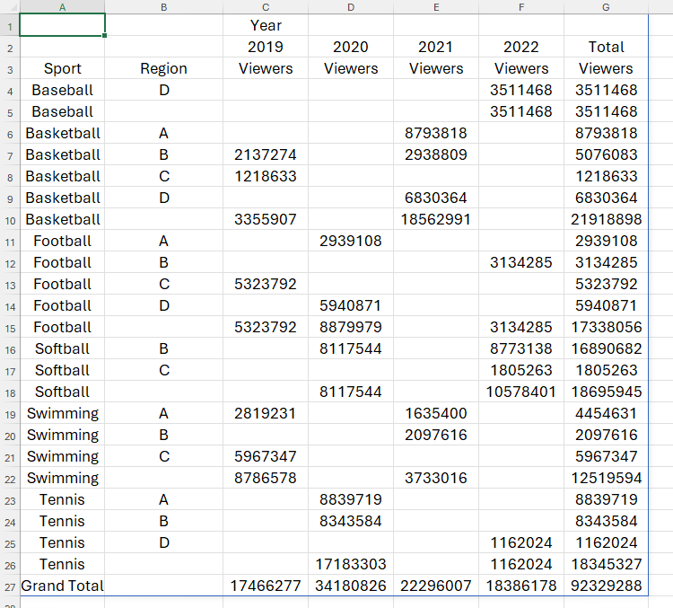
Since the PIVOTBY function does not provide an option for formatting results, it becomes challenging to differentiate between header rows, data rows, subtotal rows, and the grand total row.
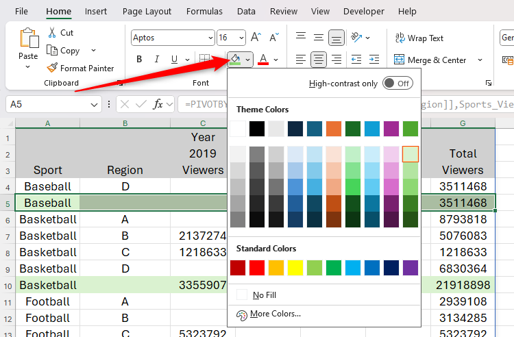
At this point, you may feel inclined to use direct formatting—from the Font section within the Home tab on the ribbon—to distinguish visually between various row types in your dataset.
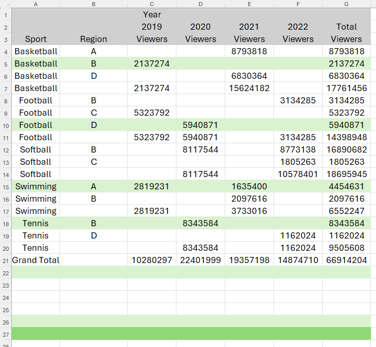
If you subsequently alter the settings within the PIVOTBY formula, or if the output expands or contracts as a result of modifications to the initial dataset, the manual formatting you've applied will not adapt appropriately. This occurs because manually set formats in Excel are tied to specific cells instead of their contents. Consider the potential for misunderstanding illustrated in the image below; here, despite the reduction in data size, the previous cell-level formatting remains unchanged across what now appears to be more rows than necessary.
Alternatively, you can utilize conditional formatting, enabling you to style the cells and rows based on their values.
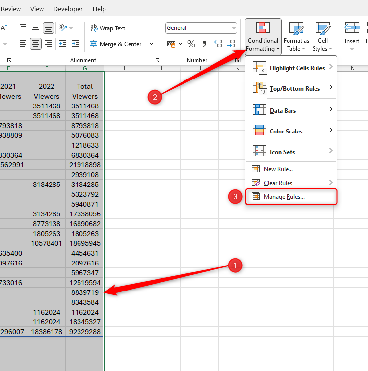
Choose all the information along with additional rows beneath to accommodate future expansion. Then go to the Home tab on the toolbar, select Conditional Formatting, and click on Manage Rules.
Next, open the Conditional Formatting Rules Manager dialog box and click "New Rule."
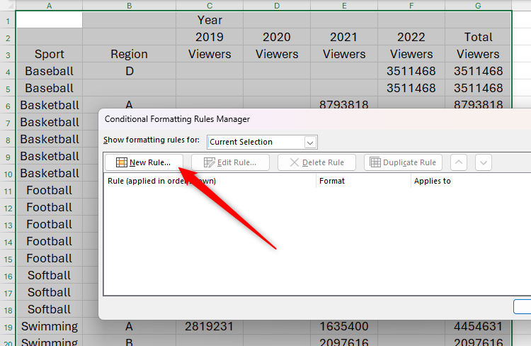
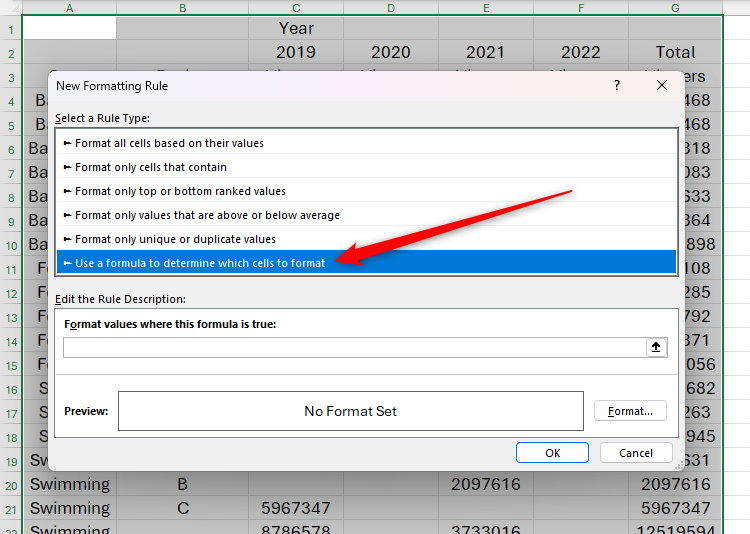
For every rule you plan to establish for formatting your scattered array, you will have to utilize a formula. Therefore, within the Select A Rule Type section of the New Formatting Rule dialogue box, choose the last option, which is "Use A Formula To Decide Which Cells Get Formatted."
The initial rule you wish to establish pertains to the header rows. You specifically want these cells to have a gray background color.
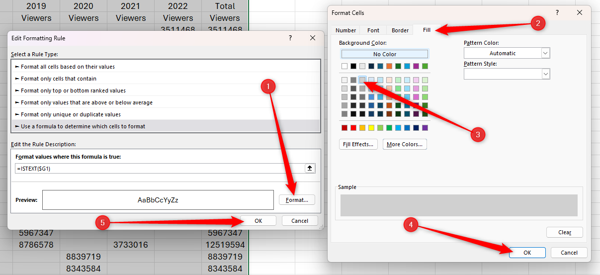
To accomplish this, spend a moment identifying what distinguishes the header rows from the rest of the rows in your table. Here, the header rows are characterized as the ones that do not have any numbers in column G. Therefore, in the formula field, enter:
=ISTEXT($G1)Since the ISTEXT function handles empty cells and those with textual content as text values; thus, the conditional formatting rule will view cells G1 through G3 as containing text, whereas the rest of the cells in column G hold numerical values.
Significantly, placing a dollar ($) symbol preceding the column reference—which is referred to as a mixed reference—locks the conditional formatting onto this specific column, permitting Excel to extend the rule across the rest of the rows.
Once you enter a cell reference, instead of adding the dollar signs by hand, hit F4 to switch among absolute references (such as $G$1), mixed references (like $G1 or G$1), and relative references (for instance, G1).
Ultimately, since you first chose data spanning from column A through column G, the conditional formatting will be applied across the entire row whenever the specified condition is fulfilled.
Next, press "Format" to choose the style for your header rows; here, they should appear with a gray coloration. Afterward, confirm your choice by clicking "OK" within both the Format Cells and Edit Formatting Rule windows.
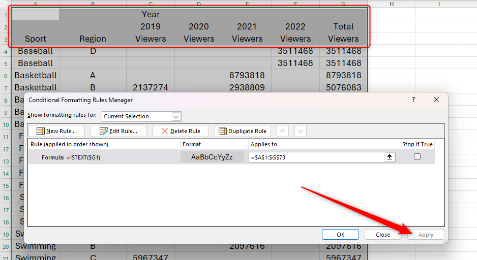
Upon clicking "Apply" within the Conditional Formatting Rules Manager dialogue box, you will notice that only those rows where column G includes empty cells or text—that being said, the header rows—will be shaded grey.
Next, you should adjust thesubtotal rows to have a light green fill.
Once more, thoroughly examine the data to determine which conditions should be applied for formatting these specific rows. Here, the subtotal lines have entries in column A yet lack content in column B. Additionally, because the grand total line fits these same parameters, ensure you omit from consideration any cell in column A with the phrase “Grand Total.”
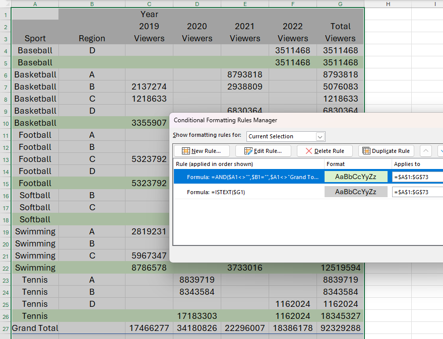
While keeping the Conditional Formatting Rules Manager dialogue box open, click “New Rule,” and choose the option that allows you to apply formatting using a formula. In this instance, enter the following formula into the designated field:
=AND($A1<>"",$B1="",$A1<>"Grand Total")where
- The AND function enables you to define multiple conditions inside the parentheses,
- $A1 < >"" tells Excel to look for cells in column A that do not contain (<>) blank cells (""),
- $B1="" instructs Excel to search for cells in column B that have blank entries ("""") within them, and
- $A1 < >"Grand Total" instructs Excel to ignore (<>) any cells in column A that include the text "Grand Total."
Just like with the preceding rule, make sure to place the $ symbol before the column identifiers so that Excel can extend this formatting across all chosen rows.
Next, select "Format" to pick the light green fill color, then close both the Format Cells and Edit Formatting Rule windows before clicking "Apply." This will display the subtotal rows with a light green background.
Ultimately, your aim is for the cells in the grand total row to appear as a deeper green, making them more prominent.
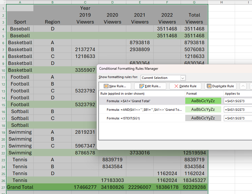
As the grand total row is distinguished by having "Grand Total" appear solely in column A, this serves as your basis for setting up conditional formatting. Within the Conditional Formatting Rules Manager dialogue box, press "New Rule", then choose the last choice listed under Select A Rule Type. Next, input the following into the formula box:
=$A1="Grand Total"Next, click “Format,” then choose a bold green fill color for applying to the cells meeting this condition. Upon closing both the Format Cells and Edit Formatting Rule windows, followed by clicking ‘Apply’ within the Conditional Formatting Rules Manager window, you will notice that your grand total row now incorporates this new style.
Once you have implemented all your conditions, click "Close" within the Conditional Formatting Rules Manager dialogue box. Next, modify some information in the initial table and observe how the changes reflect with their corresponding formatting updates.
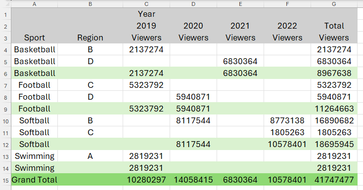
In this case, despite removing 12 rows from the initial dataset, the overflowed PIVOTBY outcome remains properly structured. The headers appear in gray, subtotals are highlighted in light green, and the grand total row stands out in bold green.
If adjustments to your established formatting rules are necessary, just pick any cell within the dataset and click Conditional Formatting > Manage Rules to reopen the Conditional Formatting Rules Manager. From there, edit a specific rule by double-clicking it.